Developing Applications
The previous section outlined most of the basic modules in the GridPACK
framework. In this section, we provide an overview of how to use these
modules to create actual applications by discussing the development of a
power flow simulation in detail. Actual examples of a power flow
application can be found by looking at an example code located under the
top-level GridPACK directory in
src/applications/examples/powerflow. Users can also look at the
power flow module located in the src/applications/modules/powerflow
directory. The main difference between the power flow example code and
the power flow module is that the module breaks up the power flow
calculation into more separate function calls and the module also has
options for using a non-linear solver. The power flow bus and branch
classes are located in the directory
src/applications/components/pf_matrix.
A schematic of a power flow code based on GridPACK is shown in Figure 8. For different power grid problems, the details of the code will be different, but most of these motifs will appear at some point or other. The main differences will probably be in feedback loops as results from one part of the calculation are fed back into other parts. For example, an iterative solver will need to update the current values of the network components, which can then be used to generate new matrices and vectors that are fed back into the next iteration of the solver. The diagram in Figure & is not complete, but gives an overall view of code structure and data movement.
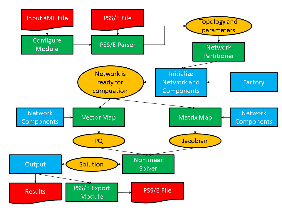
Figure 8: Schematic of program flow for a power flow simulation. The yellow ovals are distributed data objects, the green blocks are GridPACK framework components and the blue blocks are application specific code. External files are red.
As shown in the figure, application developers will need to focus on writing two or three sets of modules. The first is the network components. These are the descriptions of the physics and/or measurements that are associated with buses and branches in the power grid network. The network factory is a module that initializes the grid components on the network after the network is originally created by the import module. The power flow problem is simple enough that it can use a non-linear solver directly from the math module but even a straightforward solution such as this requires the developer to overwrite some functions in the factory that are used in the non-linear solver iterations.
Most of the work involved in creating a new application is centered on creating the bus and branch classes. This discussion will describe in some detail the routines that need to be written in order to develop a working power flow simulation. Additional application modules for dynamic simulation and contingency analysis have also been included in the distribution and users are encouraged to look at these modules for additional coding examples on how to use GridPACK. The discussion below is designed to illustrate how to build an application and for brevity has left out some code compared to the working implementation. The source code contains more comment lines as well as some additional diagnostics that may not appear here. However, the overall design is the same and readers who have a good understanding of the following text should have no difficulty understanding the power flow source code.
For the power flow calculation, the buses and branches will be
represented by the classes PFBus and PFBranch.
PFBus inherits from the BaseBusComponent class, so it
automatically inherits the BaseComponent and
MatVecInterface classes as well. The first thing that must be
done in creating the PFBus component is to overwrite the load
function in the BaseComponent class. The original function is
just a placeholder that performs no action. The load function
should take parameters from the DataCollection object associated
with each bus and use them to initialize the bus component itself. For
the PFBus component, a simplified load function is
void gridpack::powerflow::PFBus::load(
    const boost::shared_ptr<gridpack::component
    ::DataCollection> &data)
{
  data->getValue(CASE_SBASE, &p_sbase);
  data->getValue(BUS_VOLTAGE_ANG, &p_angle);
  data->getValue(BUS_VOLTAGE_MAG, &p_voltage);
  p_v = p_voltage;
  double pi = 4.0*atan(1.0;
  p_angle = p_angle*pi/180.0;
  p_a = p_angle;
  int itype; data->getValue(BUS_TYPE, &itype);
  if (itype == 3) {
    setReferenceBus(true);
  }
  bool lgen;
  int i, ngen, gstatus;
  double pg, qg;
  if (data->getValue(GENERATOR_NUMBER, &ngen)) {
    for (i=0; i<ngen; i++) {
      lgen = true;
      lgen = lgen && data->getValue(GENERATOR_PG, &pg,i);
      lgen = lgen && data->getValue(GENERATOR_QG, &qg,i);
      lgen = lgen && data->getValue(GENERATOR_STAT, &gstatus,i);
      if (lgen) {
        p_pg.push_back(pg);
        p_qg.push_back(qg);
        p_gstatus.push_back(gstatus);
      }
    }
  }
}
This version of the load function has left off additional
properties, such as shunts and loads and some transmission parameters,
but it serves to illustrate how load is suppose to work. The
load method in the base factory class will run over all buses,
get the DataCollection object associated with each bus and then
call the PFBus::load method using the DataCollection
object as the argument. The parameters p_sbase, p_angle,
p_voltage are private members of PFBus. The variables
corresponding to the keys CASE_SBASE, BUS_VOLTAGE_ANG,
BUS_VOLTAGE_MAG were stored in the DataCollection object
when the network configuration file was parsed. They are retrieved from
this object using the getValue functions and assigned to
p_sbase, p_angle, p_voltage. Additional internal
variables are also assigned in a similar manner. The value of the
BUS_TYPE variable can be used to determine whether the bus is a
reference bus. As mentioned previously, the CASE_SBASE etc.
symbols are just preprocessor symbols that are defined in the
dictionary.hpp file, which must be included in the file defining
the load function. The dictionary.hpp and associated
files can be found in the src/parser directory of the GridPACK
distribution.
The variables referring to generators have a different behavior than the
bus voltage variables. A bus can have multiple generators and these are
stored in the DataCollection object with an index. The total
number of generators on the bus is also stored in the
DataCollection object with the key GENERATOR_NUMBER.
First, the number of generators is retrieved and then a loop is set up
so that all the generator variables can be accessed. The generator
parameters are stored in local private arrays. The loop shows how the
return value of the getValue function can be used to verify that
all three parameters for a generator were found. If they aren’t found,
then the generator is incomplete and the generator is not added to the
local data. The boolean return value can also be used to determine if
the bus has other properties and to set internal flags and parameters
accordingly. The load function for the PFBranch is constructed
in a similar way, except that the focus is on extracting branch related
parameters from the DataCollection object.
Both the PFBus and PFBranch classes contain an
application-specific function called setYBus that is used to set
up values in the Y-matrix. There is also a function in the powerflow
factory class that runs over all buses and branches and calls this
function. The setYBus function in PFBus is
void gridpack::powerflow::PFBus::setYBus(void)
{
  gridpack::ComplexType ret(0.0,0.0);
  std::vector<boost::shared_ptr<BaseComponent> > branches;
  getNeighborBranches(branches);
  int size = branches.size();
  int i;
  for (i=0; i<size; i++) {
    gridpack::powerflow::PFBranch *branch
      = dynamic_cast<gridpack::powerflow::PFBranch*>
        (branches[i].get());
    ret -= branch->getAdmittance();
    ret -= branch->getTransformer(this);
    ret += branch->getShunt(this);
  }
  if (p_shunt) {
    gridpack::ComplexType shunt(p_shunt_gs,p_shunt_bs);
    ret += shunt;
  }
  p_ybusr = real(ret);
  p_ybusi = imag(ret);
}
This function evaluates the contributions to the Y-Matrix associated
with buses. The real and imaginary parts of this number are stored in
the internal variables p_ybusr and p_ybusi. The
subroutine first creates the local variable ret and then gets a
list of pointers to neighboring branches from the
BaseBusComponent function getNeighborBranches. The
function then loops over each of the branches and uses the dynamic cast
function in C++ to convert the BaseComponent pointer to a
PFBranch pointer. Note that the cast is necessary since the
getNeighborBranches function only returns a list of
BaseComponent object pointers. The BaseComponent class
does not contain application-specific functions such as
getAdmittance. The getAdmittance, getTransformer
and getShunt methods return the contributions from transmission
elements, transformers, and shunts associated with the branch. These are
accumulated into the ret variable.
The reason that the getAdmittance variable has no argument while
both getTransformer and getShunt take the pointer
“this” as an argument is that the admittance contribution from
simple transmission elements is symmetric with respect to whether or not
the calling bus is the “from” or “to” buses while the transformer and
shunt contributions are not. This can be seen by examining the
getTransformer function.
gridpack::ComplexType
  gridpack::powerflow::PFBranch::getTransformer(
    gridpack::powerflow::PFBus *bus)
{
  gridpack::ComplexType ret(p_resistance,p_reactance);
  if (p_xform) {
    ret = -1.0/ret;
    gridpack::ComplexType a(cos(p_phase_shift),sin(p_phase_shift));
    a = p_tap_ratio*a;
    if (bus == getBus1().get()) {
      ret = ret/(conj(a)*a);
    } else if (bus == getBus2().get()) {
      // ret is unchanged
    }
  } else {
    ret = gridpack::ComplexType(0.0,0.0);
  }
  return ret;
}
The variables p_resistance, p_reactance,
p_phase_shift, and p_tap_ratio are all internal
variables that are set based on the variables read in from using the
load method or are set in other initialization steps. The
boolean variable p_xform variable is set to true in the
PFBranch::load method if transformer-related variables are
detected in the DataCollection objects associated with the
branch, otherwise it is false.
The PFBranch version of the setYBus function is
void gridpack::powerflow::PFBranch::setYBus(void)
{
  gridpack::ComplexType ret(p_resistance,p_reactance);
  ret = -1.0/ret;
  gridpack::ComplexType a(cos(p_phase_shift),sin(p_phase_shift));
  a = p_tap_ratio*a;
  if (p_xform) {
    p_ybusr_frwd = real(ret/conj(a));
    p_ybusi_frwd = imag(ret/conj(a));
    p_ybusr_rvrs = real(ret/a);
    p_ybusi_rvrs = imag(ret/a);
  } else {
    p_ybusr_frwd = real(ret);
    p_ybusi_frwd = imag(ret);
    p_ybusr_rvrs = real(ret);
    p_ybusi_rvrs = imag(ret);
  }
  gridpack::powerflow::PFBus *bus1 =
    dynamic_cast<gridpack::powerflow::PFBus*>(getBus1().get());
  gridpack::powerflow::PFBus *bus2 =
    dynamic_cast<gridpack::powerflow::PFBus*>(getBus2().get());
  p_theta = (bus1->getPhase() - bus2->getPhase());
}
Note that the branch version of the setYBus function calculates
different values Y-matrix contribution for the forward and reverse
directions, where forward and reverse are defined depending on whether
the first index in the Y-matrix element corresponds to bus 1 (the
forward direction) or bus 2 (the reverse direction). These are stored in
the separate variables p_ybusr_frwd and p_ybusi_frwd for
the forward direction and p_ybusr_rvrs and p_ybusi_rvrs
for the reverse direction. This routine also calculates the variable
p_theta which is equal to the difference in the phase angle
variable associated with the two buses at either end of the branch. This
last variable provides an example of calculating a branch parameter
based on the values of parameters located on the terminal buses.
The setYBus functions are used in the power flow components to
set some basic parameters that eventually incorporated into the Jacobian
matrix and PQ vector. These constitute the matrix and right hand side
vector of the power flow equations. To build the matrix, it is necessary
to implement the matrix size and matrix values functions in the
MatVecInterface. The functions for setting up the matrix are
discussed in detail below, the vector functions are simpler but follow
the same pattern. The mode used for setting up the Jacobian matrix is
“Jacobian”. The corresponding matrixDiagSize routine is
bool gridpack::powerflow::PFBus::matrixDiagSize(int *isize,
     int *jsize) const
{
  if (p_mode == Jacobian) {
    *isize = 2;
    *jsize = 2;
    return true;
  } else if (p_mode == YBus) {
    *isize = 1;
    *jsize = 1;
    return true;
  }
}
This function handles two modes, stored in the internal variable
p_mode. If the mode equals Jacobian, then the function
returns a contribution to a 2\(\mathrm{\times}\)2 matrix. In the
case that the mode is “YBus” the function would return a
contribution to a 1\(\mathrm{\times}\)1 matrix. (The Jacobian is
treated as a real matrix where the real and complex parts of the problem
are treated as separate variables, the Y-matrix is handle as a regular
complex matrix). The corresponding code for returning the diagonal
values is
bool gridpack::powerflow::PFBus::matrixDiagValues(ComplexType *values)
{
  if (p_mode == YBus) {
    gridpack::ComplexType ret(p_ybusr,p_ybusi);
    values[0] = ret;
    return true;
  } else if (p_mode == Jacobian) {
    if (!getReferenceBus()) {
      values[0] = -p_Qinj - p_ybusi * p_v *p_v;
      values[1] = p_Pinj - p_ybusr * p_v *p_v;
      values[2] = p_Pinj / p_v + p_ybusr * p_v;
      values[3] = p_Qinj / p_v - p_ybusi * p_v;
      if (p_isPV) {
        values[1] = 0.0;
        values[2] = 0.0;
        values[3] = 1.0;
      }
      return true;
    } else {
      values[0] = 1.0;
      values[1] = 0.0;
      values[2] = 0.0;
      values[3] = 1.0;
      return true;
    }
  }
}
In this implementation, the return values are of type
ComplexType, even if they are real. For real values, the
imaginary part is set to zero. If the mode is “YBus”, the
function returns a single complex value. If the mode is
“Jacobian”, the function checks first to see if the bus is a
reference bus or not. If the bus is not a reference bus, then the
function returns a 2\(\mathrm{\times}\)2 block corresponding to
the contributions to the Jacobian matrix coming from a bus element. If
the bus is a reference bus, the function returns a
2\(\mathrm{\times}\)2 identity matrix. This is a result of the
fact that the variables associated with a reference bus are fixed. In
fact, the variables contributed by the reference bus could be eliminated
from the matrix entirely by returning false for both the matrix size and
matrix values routines if the mode is “Jacobian” and the bus is
a reference bus. This would also require some adjustments to the
off-diagonal routines as well so that the size and matrix values
routines for off-diagonal block both return false if either end of the
branch is connected to the reference bus. There is an additional
condition for the case where the bus is a “PV” bus. In this case one of
the independent variables is eliminated by setting the off-diagonal
elements of the block to zero and the second diagonal element equal to
1. The values are returned in column-major order, so values[0]
corresponds to the (0,0) location in the 2\(\mathrm{\times}\)2
block, values[1] is the (1,0) location, values[2] is the
(0,1) location and values[3] is the (1,1) location.
The matrixForwardSize and matrixForwardValues routines,
as well as the corresponding Reverse routines, are implemented in the
PFBranch class. These functions determine the off-diagonal
blocks of the Jacobian and Y-matrix. The matrixForwardSize
routine is given by
bool gridpack::powerflow::PFBranch::matrixForwardSize(int *isize,
     int *jsize) const
{
  if (p_mode == Jacobian) {
    gridpack::powerflow::PFBus *bus1
      = dynamic_cast<gridpack::powerflow::PFBus*>(getBus1().get());
    gridpack::powerflow::PFBus *bus2
      = dynamic_cast<gridpack::powerflow::PFBus*>(getBus2().get());
    bool ok = !bus1->getReferenceBus();
    ok = ok && !bus2->getReferenceBus();
    if (ok) {
      *isize = 2;
      *jsize = 2;
      return true;
    } else {
      return false;
    }
  } else if (p_mode == YBus) {
    *isize = 1;
    *jsize = 1;
    return true;
  }
}
If the mode is “YBus”, the size function returns a
1\(\mathrm{\times}\)1 block for the off-diagonal matrix block.
For the Jacobian, this function first checks to see if either end of the
branch is a reference bus by evaluating the Boolean variable “ok”. If
neither end is the reference bus then the function returns a
2\(\mathrm{\times}\)2 block, if one end is the reference bus
then the function returns false. The false value indicates that this
branch does not contribute to the matrix. For this system, the
matrixReverseSize function is the same. For applications that
return a non-square block, the reverse function must transpose the block
dimensions relative to the forward direction.
The matrixForwardValues function is
bool gridpack::powerflow::PFBranch::matrixForwardValues(
   ComplexType *values)
{
  if (p_mode == Jacobian) {
    gridpack::powerflow::PFBus *bus1
      = dynamic_cast<gridpack::powerflow::PFBus*>(getBus1().get());
    gridpack::powerflow::PFBus *bus2
      = dynamic_cast<gridpack::powerflow::PFBus*>(getBus2().get());
    bool ok = !bus1->getReferenceBus();
    ok = ok && !bus2->getReferenceBus();
    if (ok) {
      double cs = cos(p_theta);
      double sn = sin(p_theta);
      values[0] = (p_ybusr_frwd*sn - p_ybusi_frwd*cs);
      values[1] = (p_ybusr_frwd*cs + p_ybusi_frwd*sn);
      values[2] = (p_ybusr_frwd*cs + p_ybusi_frwd*sn);
      values[3] = (p_ybusr_frwd*sn - p_ybusi_frwd*cs);
      values[0] *= ((bus1->getVoltage())*(bus2->getVoltage()));
      values[1] *= -((bus1->getVoltage())*(bus2->getVoltage()));
      values[2] *= bus1->getVoltage();
      values[3] *= bus1->getVoltage();
      bool bus1PV = bus1->isPV();
      bool bus2PV = bus2->isPV();
      if (bus1PV & bus2PV) {
        values[1] = 0.0;
        values[2] = 0.0;
        values[3] = 0.0;
      } else if (bus1PV) {
        values[1] = 0.0;
        values[3] = 0.0;
      } else if (bus2PV) {
        values[2] = 0.0;
        values[3] = 0.0;
      }
      return true;
    } else {
      return false;
    }
  } else if (p_mode == YBus) {
    values[0] = gridpack::ComplexType(p_ybusr_frwd,p_ybusi_frwd);
    return true;
  }
}
For the “YBus” mode, the function simply returns the complex
contribution to the Y-matrix. For the “Jacobian” mode, the
function first determines if either end of the branch is connected to
the reference bus. If it is, then the function returns false and there
is no contribution to the Jacobian. If neither end of the branch is the
reference bus then the function evaluates the 4 elements of the
2\(\mathrm{\times}\)2 contribution to the Jacobian coming from
the branch. To do this, the branch needs to get the current values of
the voltages on the buses at either end by using the getVoltage
accessor functions that have been defined in the PFBus class.
Finally, if one end or the other of the branch is a PV bus, then some
variables need to be eliminated from the equations. This can be done by
setting appropriate values in the 2\(\mathrm{\times}\)2 block
equal to zero.
The matrixReverseValues function is similar to the
matrixForwardValues functions with a few key differences. 1) the
variables p_ybusr_rvrs and p_ybusi_rvrs are used instead
of p_ybusr_frwd and p_ybusi_frwd 2) instead of using
cos(p_theta) and sin(p_theta) the function uses
cos(-p_theta) and sin(-p_theta) since p_theta is
defined as difference in phase angle on bus 1 minus the difference in
phase angle on bus 2 and 3) the values that are set to zero in the
conditions for PV buses are transposed. The PV conditions are the same
as the forward case if both bus 1 and bus 2 are PV buses, if only bus 1
is a PV bus then values[2] and values[3] are zero and if
only bus2 is a PV bus then values[1] and values[3] are
zero.
The functions for setting up vectors are similar to the corresponding
matrix functions, although they are a bit simpler. The vector part of
the MatVecInterface contains one function that does not have a
counterpart in the set of matrix functions and that is the
setValues function. This function can be used to push values in
a vector object back into the buses that were used to generate the
vector. For the Newton-Raphson method used to solve the power flow
equations, it is necessary to push the current solution back into the
buses at each iteration so they can be used to evaluate new Jacobian and
right hand side vectors. The solution vector contains the current
increments to the voltage and phase angle. These are written back to the
buses using the function
void gridpack::powerflow::PFBus::setValues(
    gridpack::ComplexType *values)
{
  p_a -= real(values[0]);
  p_v -= real(values[1]);
  *p_vAng_ptr = p_a;
  *p_vMag_ptr = p_v;
}
If the matrix equation Ax = b is being solved, then the mapper
used to create the right hand side vector b should be used to
push results back onto the buses using the mapToBus method. The
setValues method above takes the contributions from the solution
vector and uses then to decrement the internal variables p_a
(voltage angle) and p_v (voltage magnitude). The new values of
p_a and p_v are then assigned to the buffers
p_vAng_ptr and p_vMag_ptr so that they can be exchanged
with other buses. This is discussed below.
The two routines that need to be created in the PFBus class to
copy data to ghost buses are both simple. There is no need to create
corresponding routines in the PFBranch class since branches do
not exchange data in the power flow calculation. Two values need to be
exchanged between buses, the current voltage angle and the current
voltage magnitude. This requires a buffer that is the size of two
doubles so the getXCBufSize function is written as
int gridpack::powerflow::PFBus::getXCBufSize(void)
{
  return 2*sizeof(double);
}
The setXCBuf assigns the buffer created in the base factory
setExchange function to internal variables used within the
PFBus component. It has the form
void gridpack::powerflow::PFBus::setXCBuf(void *buf)
{
  p_vAng_ptr = static_cast<double*>(buf);
  p_vMag_ptr = p_vAng_ptr+1;
  *p_vAng_ptr = p_a;
  *p_vMag_ptr = p_v;
}
The buffer created in the setExchange routine is split between
the two internal pointers p_vAng_ptr and p_vMag_ptr.
These are then initialized to the current values of p_a and
p_v. Whenever the updateBuses routine is called, the
buffers on the ghost buses are refreshed with the current values of the
variables from the processes that own the corresponding buses. Note that
both the getXCBufSize and the setXCBuf routines are only
called during the setExchange routine. They are not called
during the actual bus updates.
One final function in the PFBus and PFBranch class that
is worth taking a brief look at is the set mode function. This function
is used to set the internal p_mode variable that is defined in
both classes. The PFMode enumeration, which contains both the
“YBus” and “Jacobian” modes, is defined within the
gridpack::powerflow namespace. The setMode function for both
buses and branches has the form
void gridpack::powerflow::PFBus::setMode(int mode)
{
  p_mode = mode;
}
This function is triggered on all buses and branches if the
setMode method in the factory class is called. Once the
PFBus and PFBranch classes have been defined, it is
possible to define a PFNetwork using a typdef statement.
This can be done using the line
typedef network::BaseNetwork<PFBus, PFBranch > PFNetwork;
in the header file declaring the PFBus and PFBranch
classes. This type can then be used in other powerflow files that need
to create objects from templated classes.
The discussion above summarizes many of the important functions in the
PFBus and PFBranch classes. Additional functions are
included in these classes that are not discussed here, but the basic
principles involved in implementing the remaining functions have been
covered.
The first part of creating a new application is writing the network
component classes. The second part is implementing the
application-specific factory. For the power flow application, this is
the PFFactory class, which inherits from the BaseFactory
class. Most of the important functionality in PFFactory is
derived from the BaseFactory class and is used without
modification, but several application-specific functions have been added
to PFFactory that are used to set internal parameters in the
network components. As an example, consider the setYBus function
void gridpack::powerflow::PFFactory::setYBus(void)
{
  int numBus = p_network->numBuses();
  int numBranch = p_network->numBranches();
  int i;
  for (i=0; i<numBus; i++) {
    p_network->getBus(i).get()->setYBus();
  }
  for (i=0; i<numBranch; i++) {
    p_network->getBranch(i).get()->setYBus();
  }
}
This function loops over all buses and branches and invokes the
setYBus method in the individual PFBus and
PFBranch objects. The first two lines in the factory
setYBus method get the total number of buses and branches on the
process. A loop over all buses on the process is initiated and a pointer
to the bus object is obtained via the getBus bus method in the
BaseNetwork class. This pointer is returned as a pointer of type
PFBus, so it is not necessary to do a dynamic cast on it and the
setYBus method, which is not part of the base class, can be
invoked. The same set of steps is then repeated for the branches. The
factory can be used to create other methods that invoke functions on
buses and/or branches.
Most of these functions follow the same general form as the
setYBus method just described. The last part of building an
application is creating the top level application driver that actually
instantiates all the objects used in the calculation and controls the
program flow. Running the code is broken up into two parts. The first is
creating a main program and the second is creating the application
driver. The main routine is primarily responsible for initializing the
communication libraries and creating the application object, the
application object then controls the application itself. The main
program for the powerflow application is
main(int argc, char **argv)
{
  gridpack::parallel::Environment env(argc,argv);
  {
    gridpack::powerflow::PFApp app;
    app.execute();
  }
}
The first line in this program creates a variable of type
Environment that initializes the MPI and GA communication
libraries as well as the math initialization routine (the initialization
happens in the constructor, so all that is necessary is to create the
variable). More can be found out about the Environment class in
Section 6.2. The code then instantiates a power flow
application object and calls the execute method for this object. The
remainder of the power flow application is contained in the
PFApp::execute method. Finally, when the application has
finished running, the main program cleans up the communication and math
libraries. The communication libraries are handled when the env
variable goes out of scope and calls the Environment destructor.
The main reason for breaking the code up in this way instead of
including the execute function as part of main is to force the
invocation of all the destructors in the GridPACK objects used to
implement the application. Otherwise, these destructors get called after
the communication libraries have been finalized and the program will
fail to exit cleanly.
The top level control of the application is embedded in the power flow
execute method. The execute method starts off with the
code
gridpack::parallel::Communicator world;
boost::shared_ptr<PFNetwork> network(new PFNetwork(world));

gridpack::utility::Configuration *config
    = gridpack::utility::Configuration::configuration();
config->open("input.xml",world);
gridpack::utility::Configuration::Cursor *cursor;
cursor = config->getCursor("Configuration.Powerflow");
std::string filename;
if (!cursor->get("networkConfiguration", &filename)) {
  printf("No network configuration specified\n");
  return;
}
gridpack::parser::PTI23_parser<PFNetwork> parser(network);
parser.parse(filename.c_str());

network->partition();
The first two lines create a communicator for this application and use
it to instantiate a PFNetwork object (note that this is really a
BaseNetwork template class that is instantiated using the
PFBus and PFBranch classes as template arguments). The
network object exists but has no buses or branches associated with it.
The next few lines get an instance of the configuration object and use
this to open the input.xml file. This filename has been
hardwired into this implementation but it could be passed in as a
runtime argument, if desired. The code then creates a Cursor
object and initializes this to point into the
Configuration.Powerflow block of the input.xml file. The
cursor can then be used to get the contents of the
networkConfiguration block in input.xml, which
corresponds to the name of the network configuration file containing the
power grid network. This file is assumed to use the PSS/E version 23
format. After getting the file name, the code creates a
PTI23_parser object and passes in the current network object as
an argument. When the parse method is called, the parser reads in the
file specified in filename and uses that to add buses and
branches to the network object. The network now has all the bus and
branches from the configuration file, but no ghost buses or branches
exist and buses and branches are not distributed in an optimal way.
Calling the partition method on the network distributes the buses and
branches and adds appropriate ghost buses and branches.
The next set of calls initialize the network components and prepare the network for computation.
gridpack::powerflow::PFFactory factory(network);
factory.load();

factory.setComponents();
factory.setExchange();

network->initBusUpdate();

factory.setYBus();
The first call creates a PFFactory object and instantiates it
with a reference to the current network. PFFactory inherits from
the BaseFactory class and assumes that a PFNetwork is
used as the template argument for the BaseFactory. The next line
calls the BaseFactory load method which invokes the component
load method on all buses and branches. These methods use data
from the DataCollection objects to initialize the corresponding
bus and branch objects. Note that when the partition function creates
the ghost bus and branch objects, it copies the associated
DataCollection objects to these ghosts so the parameters from
the network configuration file are available to instantiate all objects
in the network. There is no need to do a data exchange at this point in
the code in order to get current values on the ghost objects.
The next two calls are implemented in the BaseFactory class. The
setComponents method sets up pointers in the network components
that point to neighboring branches and buses (in the case of buses) and
terminal buses (in the case of branches). It is also responsible for
setting up internal indices that are used by the mapper functions to
create matrices and vectors. The setExchange method sets up the
buffers that are used to exchange data between locally owned buses and
branches and their corresponding ghost images on other processors. The
call to initBusUpdate creates internal data structures that are
used to exchange bus data between processors and the final factory call
to setYBus evaluates the Y-matrix contributions from all network
components. The network is fully initialized at this point and ready for
computation.
The next calls create the matrices used in the Newton-Raphson iteration loop.
factory.setSBus();
factory.setMode(RHS);
gridpack::mapper::BusVectorMap<PFNetwork> vMap(network);
boost::shared_ptr<gridpack::math::Vector> PQ = vMap.mapToVector();

factory.setMode(Jacobian);
gridpack::mapper::FullMatrixMap<PFNetwork> jMap(network);
boost::shared_ptr<gridpack::math::Matrix> J = jMap.mapToMatrix();
boost::shared_ptr<gridpack::math::Vector> X(PQ->clone());
The factory calls the setSBus method that sets some additional
network component parameters used in the RHS vector (again, by looping
over all buses and invoking a setSBus method on each bus). The
next three lines set the mode to “RHS”, create a
BusVectorMap object and create the right hand side vector in the
powerflow equations using the mapToVector method. This builds
the vector based on the “RHS” mode. The next three lines create
the Jacobian using the same pattern as for the Y-matrix. The mode gets
set to “Jacobian”, another FullMatrixMap object is
created and this is used to create the Jacobian using the
mapToMatrix method. The last line creates a new vector by
cloning the PQ vector. The X vector has the same dimension and data
layout as PQ so it could be used with the vMap object.
This application only creates one matrix so only one
FullMatrixMap object is needed. If multiple matrices are
required by an application then multiple FullMatrixMap objects
may need to be created, one for each matrix. In the case that multiple
matrices have exactly the same dimensions and fill pattern, it may be
possible to reuse a mapper for more than one matrix, but this will
generally not be the case.
Once the vectors and matrices for the problem have been created and set to their initial values, it is possible to start the Newton-Raphson iterations. The code to set up the first Newton-Raphson iteration is
double tolerance = 1.0e-6;
int max_iteration = 100;
ComplexType tol;

gridpack::math::LinearSolver solver(*J);
solver.configure(cursor);

int iter = 0;

X->zero();
solver.solve(*PQ, *X);
tol = PQ->normInfinity();
The first three lines define some parameters used in the Newton-Raphson
loop. The tolerance and maximum number of iterations are hardwired in
this example but could be made configurable via the input deck using the
Configuration class. The next line creates a linear solver based
on the current value of the Jacobian, J. The call to the
configure method allows configuration parameters in the input file to be
passed directly to the newly created solver. The iteration counter is
set to zero and the value of X is also set to zero. The linear
solver is called with PQ as the right hand side vector and
X as the solution. An initial value of the tolerance is set by
evaluating the infinity norm of PQ. The calculation can now
enter the Newton-Raphson iteration loop
while (real(tol) > tolerance && iter < max_iteration) {
  factory.setMode(RHS);
  vMap.mapToBus(X);
  network->updateBuses();

  vMap.mapToVector(PQ);
  factory.setMode(Jacobian);
  jMap.mapToMatrix(J);

  X->zero();
  solver.solve(*PQ, *X);
  tol = PQ->normInfinity();
  iter++;
}
This code starts by pushing the values of the solution vector back on to
the buses using the same mapper that was used to create PQ. The
network then calls the updateBus routine so that the ghost buses
have new values of the voltage angle and magnitude parameters from the
solution vector. New values of the Jacobian and right hand side vector
are created based on the solution values from the previous iteration.
Note that since J and PQ already exist, the mappers are
just overwriting the old values instead of creating new data objects.
The linear solver is already pointing to the Jacobian matrix so it
automatically uses the new Jacobian values when calculating the solution
vector X. If the norm of the new PQ vector is still
larger than the tolerance, the loop goes through another iteration. This
continues until the tolerance condition is satisfied or the number of
iterations reaches the value of max_iteration.
If the Newton-Raphson loop converges, then the calculation is essentially done. The last part of the calculation is to write out the results. This can be accomplished using the code
factory.setMode(RHS);
vMap.mapToBus();
network->updateBuses();

gridpack::serial_io::SerialBusIO<PFNetwork> busIO(128,network);
busIO.header("\n   Bus Voltages and Phase Angles\n");
busIO.header("\n   Bus Number      Phase Angle");
busIO.header("      Voltage Magnitude\n");
busIO.write();
The first three lines guarantee that current values of the solution
vector are available on all buses. The final five lines create a serial
bus IO object that assumes that no line of output will exceed more than
128 characters, write out the header for the output data and then write
a listing of data from all buses. The data from each bus is generated by
the serialWrite method defined in the PFBus class. A
similar set of calls can be used to write out data from the branches.
This completes the execute method and the overview of the power flow
application.